How to freeze a row in excel

 4.5/5

Want create site? Find Free WordPress Themes and plugins.

To freeze a row in Excel, ensuring it remains visible as you scroll through your spreadsheet, first select the row immediately below the row you want to freeze. For example, if you want to freeze the first row, select the second row. Then, go to the “View” tab in the ribbon at the top of Excel, and click on “Freeze Panes” in the Window group. From the drop-down menu, choose “Freeze Panes” again. This action locks the row above your selection, keeping it visible as you navigate the rest of your worksheet. If you want to unfreeze the row later, simply return to the “View” tab, click on “Freeze Panes,” and select “Unfreeze Panes.”

Understanding Freezing Panes in Excel
When to Use Frozen Rows
Step-by-Step Guide to Freeze a Row
Tips and Tricks for Using Frozen Rows
Conclusion
FAQs

Understanding Freezing Panes in Excel

Freezing panes in Excel is a useful feature that allows you to keep certain rows or columns visible while you scroll through the rest of your spreadsheet. Here are some key points to understand about freezing panes:

Purpose of Freezing Panes: The primary purpose of freezing panes is to lock specific rows or columns in place. This is especially helpful when working with large datasets where headers or key fields need to remain visible to maintain context as you scroll down or across the spreadsheet.
How to Freeze Panes:

To freeze rows, select the row below where you want the freeze to start. For columns, select the column to the right of where you want the freeze to start.
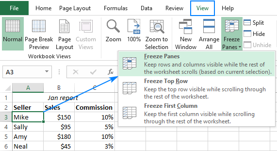
Go to the “View” tab on the Excel ribbon, click on “Freeze Panes” in the Window group, and then choose “Freeze Panes” from the drop-down menu.

3. Freezing Multiple Rows or Columns: You can freeze both rows and columns at the same time by selecting a cell that is below the rows and to the right of the columns you want to freeze. Then, follow the same steps to freeze panes.

4. Freezing the Top Row or First Column: Excel offers a shortcut for freezing the top row or the first column of the worksheet. Under the “Freeze Panes” button, select “Freeze Top Row” or “Freeze First Column” if you quickly want to lock just the first row or column.

5. Unfreezing Panes: To unfreeze rows or columns, go back to the “View” tab, click on “Freeze Panes,” and then select “Unfreeze Panes.” This will remove any frozen panes and allow the entire worksheet to scroll freely.

6. Viewing and Navigating: When panes are frozen, the line between frozen and unfrozen areas becomes slightly thicker, indicating the division. This visual marker helps in understanding which parts of the spreadsheet are fixed while scrolling.

When to Use Frozen Rows

Using frozen rows in Excel is particularly advantageous in several specific scenarios to enhance the readability and functionality of a spreadsheet. Here are key situations where freezing rows can be beneficial:

Data Entry and Review: When entering or reviewing large sets of data, freezing the top row(s) that contain headers allows you to keep track of which data goes under which column. This is crucial for maintaining accuracy and consistency in data entry, especially when dealing with extensive lists.
Financial and Statistical Analysis: In spreadsheets containing financial statements, budgets, or statistical data, it’s helpful to freeze header rows that describe the content below them. This ensures that as you scroll through rows of numbers, you can always see the column titles, which aids in interpreting and analyzing data correctly.
Comparing Data Across a Wide Range: If you need to compare or cross-reference data that spans many rows, freezing the top row(s) allows you to keep the labeling information in view while scrolling through the data. This makes comparisons quicker and reduces errors from losing track of which data belongs to which category.
Presentations and Meetings: During presentations or meetings where Excel data is shared on a screen, having the header rows frozen ensures that everyone can follow along easily as the data is scrolled through. This keeps the context visible, enhancing comprehension and engagement.
Large Reports and Datasets: For reports that span multiple pages or datasets that continue beyond the screen view, freezing the header rows is essential for navigating the data without losing sight of what each column represents. It helps maintain orientation within the spreadsheet.
Dashboard and Tracking Systems: When Excel is used to create dashboards or track projects, key metrics often need to be constantly visible at the top. Freezing these rows can help users quickly reference critical data points without having to scroll up repeatedly.

Step-by-Step Guide to Freeze a Row

Freezing a row in Microsoft Excel ensures that it remains visible as you scroll through your document, which can be incredibly useful for keeping headers displayed. Here’s a step-by-step guide on how to freeze a row in Excel:

Open Your Excel Workbook: Start by opening the Excel file where you want to freeze a row.
Select the Row Below: Click on the row number just below the row you wish to freeze. For example, if you want to freeze the first row of your spreadsheet, click on the second row. This action ensures that the row above (the one you want to freeze) stays visible as you scroll down.
Navigate to the View Tab: Look at the top of the Excel window for the ribbon and find the “View” tab. Click on it to open the view options.
Click on Freeze Panes: In the “Window” group on the “View” tab, you will see the “Freeze Panes” button. Click on this button to open a dropdown menu.
Choose ‘Freeze Panes’: From the dropdown menu, there are a few options: “Freeze Panes,” “Freeze Top Row,” and “Freeze First Column.” Since you want to freeze a specific row, choose “Freeze Panes.” This option will freeze the rows above and any columns to the left of your selected cell.
Confirm the Freeze: After clicking “Freeze Panes,” a line will appear below the row that is frozen, indicating that the row above will remain on screen as you scroll through the rest of your spreadsheet.
Test the Freeze: Scroll down your worksheet to ensure that the frozen row remains visible as other data move up and down.
Adjust if Necessary: If the wrong row is frozen or you want to change the frozen area, you can unfreeze by going back to the “Freeze Panes” button and selecting “Unfreeze Panes.” You can then repeat the above steps to freeze the correct row.

Tips and Tricks for Using Frozen Rows

Using frozen rows effectively in Excel can greatly enhance your spreadsheet management and data viewing experience. Here are some tips and tricks to get the most out of this feature:

Freeze Multiple Rows: If you have more than one header row or if several top rows contain crucial information, you can freeze all of them at once. Just select the row below the last row you want frozen, and then apply the freeze panes command.
Use Keyboard Shortcuts: To speed up your workflow, you can use shortcuts to quickly freeze panes. After selecting the row, you can press Alt + W + F + F on your keyboard to freeze the panes directly without navigating through the menus.
Combine Frozen Rows with Filters: If your frozen rows include headers for columns that you want to filter or sort, you can apply Excel’s filter functionality to these headers. This allows you to keep headers in view while filtering or sorting the data below them.
Freeze Rows for Large Datasets: When working with large datasets that extend beyond one screen, freezing the header rows allows you to maintain context as you analyze or enter data, reducing the likelihood of input errors and improving efficiency.
Remember to Unfreeze: Before rearranging rows or performing major changes that involve the insertion or deletion of rows, remember to unfreeze panes. This prevents confusion about which rows are frozen and ensures that changes are applied correctly throughout the document.
Utilize Split Panes for Comparison: If you need to compare data from different parts of the same worksheet, consider using the “Split” option instead of or in addition to “Freeze Panes.” Splitting the window allows you to scroll independently in different sections of the worksheet, making comparisons easier without losing sight of key data.
Monitor Performance: Keep in mind that freezing a large number of rows and columns might impact the scrolling performance of your worksheet, especially in very large files. If you experience slowdowns, try reducing the number of frozen panes or optimizing your spreadsheet.
Double Check Print Layout: Frozen panes affect only what you see on the screen, not how a spreadsheet prints. Use “Print Titles” under the Page Layout tab to repeat header rows on every page when printing large tables.

Conclusion

In conclusion, utilizing frozen rows in Excel is a powerful technique for enhancing data visibility and productivity. By freezing rows containing headers or critical information, users can maintain context while navigating through extensive datasets. This feature is particularly beneficial for data entry, analysis, and presentations where clarity and efficiency are paramount. Remembering to unfreeze rows as needed and exploring additional functionalities like splitting panes can further optimize your Excel workflow. With these practices, users can leverage frozen rows to streamline spreadsheet management and improve overall data handling capabilities.

FAQs

Q: 1Why should I freeze a row in Excel?

Ans:: Freezing a row in Excel allows you to keep certain rows, typically headers or labels, visible as you scroll through large amounts of data. This helps maintain context and makes it easier to work with extensive spreadsheets without losing track of important information.

Q: 2How do I freeze a row in Excel?

Ans: To freeze a row, first select the row just below the one you want to freeze. Then, go to the “View” tab on the Excel ribbon, click on “Freeze Panes” in the Window group, and choose “Freeze Panes” from the dropdown menu. This action locks the rows above your selection in place.

Q:3 Can I freeze multiple rows in Excel?

Ans: Yes, you can freeze multiple rows in Excel by selecting the row below the last row you want to freeze. Follow the same steps as freezing a single row, and all selected rows above will remain visible as you scroll through your spreadsheet.

Q: 4 How do I unfreeze rows in Excel?

Ans: To unfreeze rows, go back to the “View” tab, click on “Freeze Panes” in the Window group, and select “Unfreeze Panes” from the dropdown menu. This removes the frozen panes and allows your spreadsheet to scroll freely.

Did you find apk for android? You can find new Free Android Games and apps.